Most of the popular language models are Transformer-based architectures that use an important technique called 'self-attention'. The 'self-attention' is a little different from the attention mechanism used in the RNN-based encoder-decoder model. Let's first try to understand the intuition before delving into mathematical details and equations.
The primary function of self-attention is to generate context-aware vectors from the input sequence itself rather than considering both input and output as in the RNN-based encoder-decoder architecture. See the example below shown in Fig. 1 (Ref. Deep Learning with Python by François Chollet).
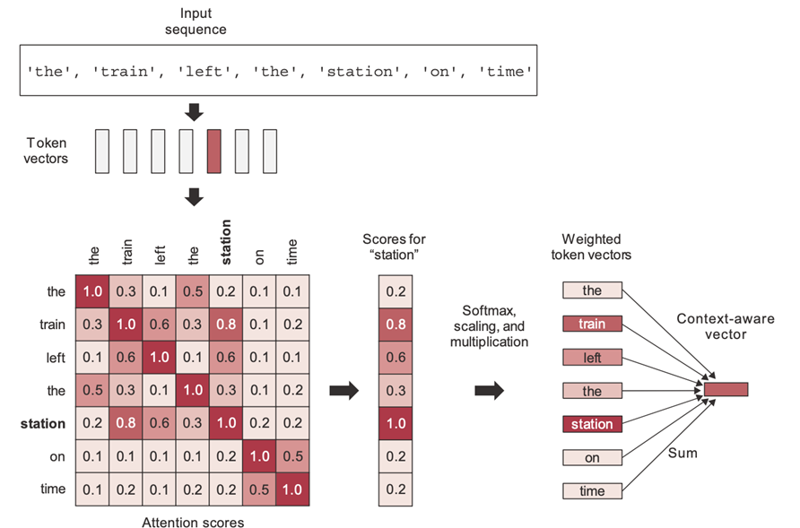
Figure 1
In this example, there are 7 sequences in the sentence 'the train left the station on time', and we can see there is a 7x7 attention score matrix. For the time being, let's say we somehow obtained these attention score values.
According to the self-attention scores depicted in the picture, the word 'train' pays more attention to the word 'station' rather than other words in consideration, such as 'on' or 'the'. Alternatively, we can say the word 'station' pays more attention to the word 'train' rather than other words in consideration, such as 'on' or 'the'.
The attention scores of each word in a sequence with all other words can be calculated, and the same is shown in the figure as a 7x7 score matrix. The self-attention model allows inputs to interact with each other (i.e., calculate the attention of all other inputs with one input).
Attention scores help in understanding the contextual meaning of a word in a given sentence. For example, here the word 'station' has been used in the context of a train station, not in other contexts like a gas station or a bus station, etc.
The attention score is computed through cosine similarity, i.e., the dot product of two-word vectors, which assesses the strength of their relationship or the degree of similarity between the words being compared. Obviously, there are many other mathematical aspects to consider, which will be discussed subsequently.
These attention scores are utilized as weights for calculating the weighted sum of all the words in the sentence. For example, when representing the word 'station', the words closely related to 'station' will contribute more to the sum (including the word 'station' itself), while irrelevant words will contribute almost nothing. The resulting vector serves as a new representation for 'station': one that incorporates the surrounding context. Specifically, it includes part of the 'train' vector, thereby clarifying that it is, indeed, a 'train station'.
Let’s understand the above paragraph by writing a mathematical equation as given below, where \( A(i) \), \(\alpha(i,j)\) are weighted sum (termed as attention vector) and attention scores (weights) respectively, and individual word vectors are represented by \(x_j\). The ‘\(T_x\)' represents the total number of terms in the sequence.
\( A(i) = \sum_{j=1}^{T_x} \alpha(i,j) x_j \)Unfolding above equation, when i is equal to a word 'train' i.e. , i = train:
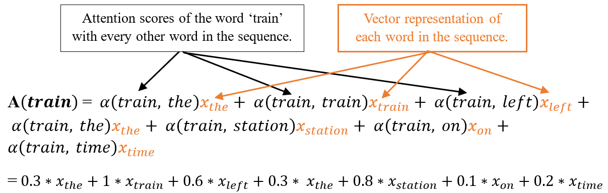
This process is iterated for every word in the sentence, yielding a new sequence of vectors that encode the sentence.
Calculation of Attention weights
Before delving into the mathematical details of the self-attention mechanism, let's revisit the equations and terms derived from the attention mechanism in RNN-based encoder-decoder architectures (as explained in my initial article: 'Birth of Attention Mechanism'). Although it's not necessary, to begin with the RNN-based attention mechanism to grasp self-attention, comparing term by term would facilitate comprehension and help us understand how identical concepts are used in both.
A conceptual diagram is shown in Fig. 2 below to depict the attention mechanism in the RNN-based encoder-decoder model, where symbols have their usual meaning.
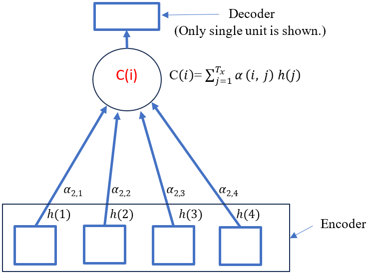
Figure 2
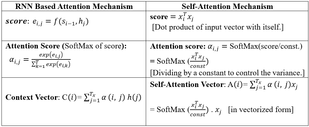
Recall, in case of Attention in RNN based encoder-decoder model:
Context vector: \( C(i)=\sum_{j=1}^{T_x} \alpha_{i,j}h(j) \)
score: \( e_{i,j} = f( S_{i-1}, h_j ) \)
Attention Score (SoftMax of score): \( \alpha_{i,j} = \frac{ \exp(e_{i,j})}{\sum_{k=1}^{T} \exp(e_{i,k})} \)
In Self-Attention, we get rid of RNN units and calculate the context-aware vectors from the input sequence itself. A conceptual diagram is shown in Fig. 3 below to depict the Self-attention. Suppose we have a sequence of feature vectors (embeddings) \( X_1 \), \( X_2 \) all the way up to \( X_T \), in this case, T equals 4. We can use the concept of cosine similarity, which measures sameness or relatedness, to calculate scores and finally obtain the SoftMax, which can be used in the context vector as given below.
In case of Self attention, score is cosine similarity, i.e. dot product of input sequence with itself.
Thus,
score: \( X_i ^{T}. X_j \); [Dot product of input vector with itself.]
Attention Score: \( \alpha_{i,j} = SoftMax(score/const.) \) [Dividing by a constant to control the variance]
Self-Attention Vector: \( A(i)=\sum_{j=1}^{T_x} \alpha_{i,j}x(j) \)
Here, h(j) is replaced by \( x_j \) and notation is changed from C to A as we call it 'Attention Vector' instead of 'context vector'.
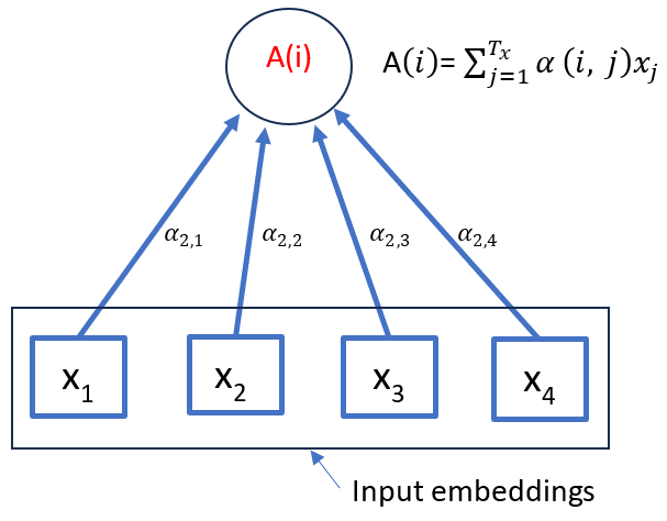
Figure 3
Self-Attention in vectorized form: \( SoftMax( \frac{X_i ^{T}. X_j } {const.}). x_j \) ---------(I)
Table 1 shown below presents the side-by-side comparison of Self Attention Mechanism and RNN based Attention Mechanism.
Table 1: Comparison of Self attention and RNN based Attention
Introducing Queries(Q), Keys(K), and Values(V)
We computed the Self-Attention vector, as derived above, based on the inputs of the vectors themselves.
This means that for fixed inputs, these attention weights would always be fixed. In other words, there are no learnable parameters. This is problematic and needs to be fixed by introducing some learnable parameters that will make the self-attention mechanism more flexible and tunable for various tasks. To fulfill this purpose, three trainable weight matrices are introduced and multiplied with input \( X_i \) separately, and three new terms Queries(Q), Keys(K), and Values(V) come into the picture as given by the equations below. Vectorized implementation & Shape tracking are also shown in subsequent steps.
Assume input 'X' is a sequence of 'T' time steps or in simple words a sentence with 'T' words and each word is represented by an Embedding vector of dimension ' \( d_{model} \) '. Fig. 4 below is showing multiple sentence samples (Xi's) in rows S1, S2, S3, and so on, and words by column as ti=1, 2, 3, ..., ti=T, which is say, up to 100.
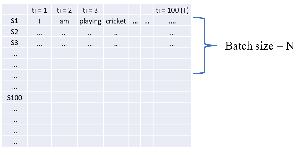
Figure 4
shape of \( X \rightarrow T \times d_{model} \)
\( d_{model} \) = Embedding vector for each word (512 as per the paper)
Queries: \( Q = XW^Q \); Where \( W^Q \) is weight matrix introduced to calculate Q from X.
Keys: \( K = XW^K \); Where \( W^K \) is weight matrix introduced to calculate K from X.
Values: \( V = XW^V \); Where \( W^V \) is weight matrix introduced to calculate V from X.
Shape tracking → (shape of X ) Matrix multiplication (shape of Weight Matrix ) → Output shape
\( Q = XW^Q \rightarrow (T \times d_{model})* (d_{model} × d_k) \rightarrow (T \times d_k) \)
\( K = XW^K \rightarrow (T \times d_{model})* (d_{model} × d_k) \rightarrow (T \times d_k) \)
\( V = XW^V \rightarrow (T \times d_{model})* (d_{model} × d_v) \rightarrow (T \times d_v) \)
Finally, substituting Q, K, V, and const. \( = \sqrt{d_k} \) ( \( d_k \) dimensionality of the key vector) in above self-attention eqn. (I), we get equation for attention as given below:
Attention(Q,K,V) = \( SoftMax( \frac{QK^{T}} {\sqrt{d_k}})V \) ---------(II)
Fig.5 below is a graphical representation of obtaining Q, K, and V from input X and feeding into equation (II) above.
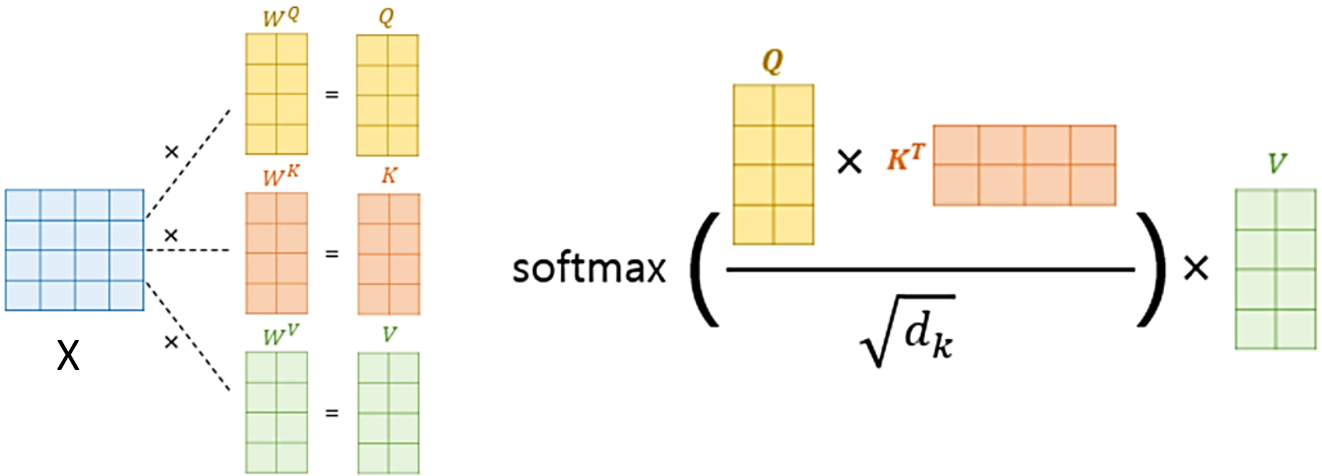
Figure 5
Above attention eqn. (II) is also termed as Scaled Dot Product Attention depicted by Fig. 6 given below.
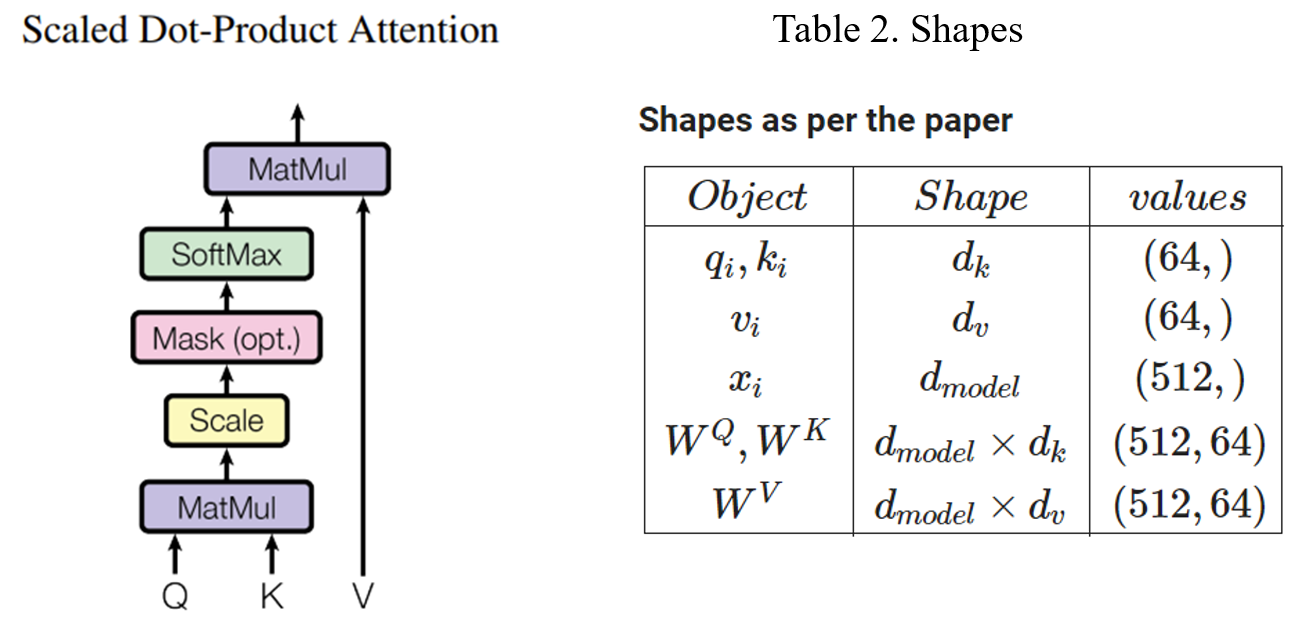
Figure 6
And finally, the shape of final attention output: \( (T \times T) * (T \times d_v) → (T \times d_v) \)
If we consider a batch of N samples at a time for processing, then above shape will be: \( N \times T \times d_v \).
Please note that the shapes of \( W^Q, W^K, W^V \) are chosen in a way that matrix multiplication with input 'X' is possible. The values of \( d_k, d_v , d_{model} \) are hyperparameters and the table of shapes above shows the values used by the author in the paper.
Database Analogy for Queries(Q), Keys(K) and Values(V)
In the context of databases, queries are used to interact with databases to retrieve or manipulate data, keys are used to uniquely identify records and establish relationships between tables, and values are the actual data stored in the fields of a database table. The same kind of analogy exists in Self-attention Q, K, and V as well, as shown in Fig. 7 below.
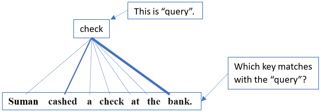
Figure 7
In self-attention, every word acts as a query once, while the entire words in the sequence act as keys, and attention weights are calculated to figure out which key matches with the query.
Finally, the words (represented as vectors) are treated as values, and attention weights are used to form a weighted sum of the values, resulting in an attention vector. The attention vector for the word 'check' will be the weighted sum of the value vectors.
How does self-attention help in contextual understanding?
In the example we looked at, we were figuring out the meaning of a word. So, if we just see the word 'check' by itself, it could mean different things. But when we look at the other words in the sentence, like 'cashed' and 'bank', it helps us understand that in this context 'check' refers to a financial document, not something like checking your homework or check in chess.
A few points to notice:
- Every word must have an attention weight with every other word, i.e., for T number of terms, T² computations are required to calculate attention weights.
- Q, K, and V are calculated independently, resulting in parallelization, unlike in RNN where h(t-1) must be computed before h(t).
- Self-attention can handle sequences of any length, unlike RNN, which has trouble with vanishing gradients.