We have discussed about discrete distributions in previous article and in discrete distributions, the events always form a list. For example, if I roll a die, I could get 1, 2, 3, 4, 5, or 6. I could also think of the number of books in a library; it can be 1, 2, 3, a thousand, etc., but I can always make a list of it.
What is something that cannot be listed? An interval. For example, if my random variable is the actual length of a manufactured shaft, that cannot be listed. Because the nominal length of the shaft is 100 mm, but it could also be 99.91 mm, or 100.01 mm, or 100.001 mm. Actually, it depends on the precision of the measuring device and up to what decimal digits we are measuring the accuracy, resulting in infinitely many values. However, we can define an interval and say that the shaft length lies between 99.90 mm and 100.10 mm.
So, when your events are a list, you have a discrete distribution. And when your events are an interval, you have a continuous distribution. Let’s elaborate more on that.
So, imagine you're measuring the length of different shafts and you're trying to find the probability that a shaft will have a specific length. Let's say the length could be exactly 99.90 mm, 100.00 mm, or 100.10 mm, for example. And we can try to plot the probabilities, say like this, where the heights of the bars are the probabilities that the length is exactly 99.90 mm, 100.00 mm, or 100.10 mm.
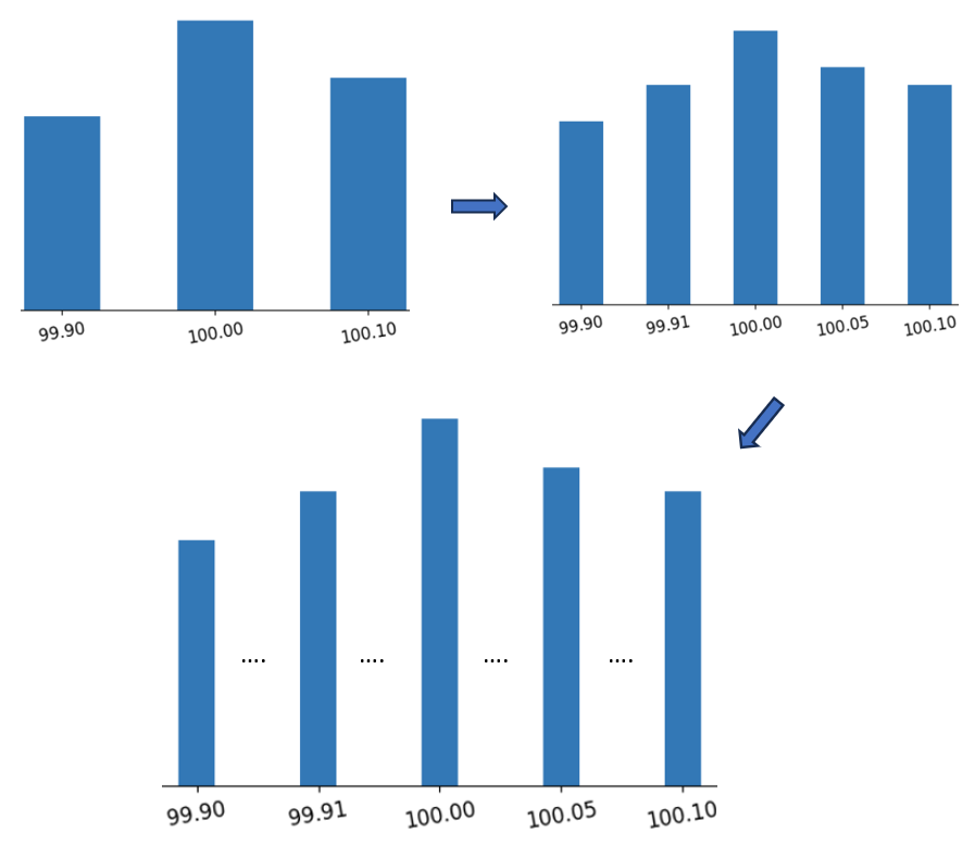
Figure 1
But it can also be 99.91 mm, or 100.05 mm. And you can quickly see that there are infinitely many values the length could take, as values with three or more decimal places are also possible. These values lie everywhere between the ones you already have, both to the left and to the right.
Since height of the bars are representing probabilities the sum of the heights of all of them has to be equal to 1. But you can quickly see that by adding more and more and more of them, they have to get smaller and smaller and eventually become 0. So, what did we do wrong here? Well, we did nothing wrong. The answer is that this distribution is fundamentally different, as it's not discrete, but it is continuous. So this approach will not really work.
To try to understand this, think of how you would answer the following question: what is the probability that the length will be exactly 100.00 mm to the dot? It is encouraged to think about this. The answer is zero, because there are simply too many values for the length. There's actually uncountably many of them; it's a whole interval. And we're forced to say that the probability that the length is exactly 100.00 and forever 0 mm is 0. So, we need to describe this problem in a slightly different way.
Instead of asking what is the probability of the length being a fixed value, let's think of it in terms of ranges. So, we're thinking of what's the probability that the length falls within a certain range, say between 99.90 and 99.95 mm. And for that, we can have a probability, and we can put it as the height of this red bar over here. Then we can think of the probability that the length falls between 99.95 and 100.00 mm. And that's this other height, or between 100.00 and 100.05 mm, and so on
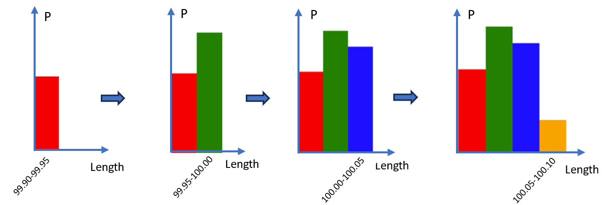
Figure 2
And let's assume that we are only considering lengths between 99.90 and 100.10 mm. And now we have a discrete probability distribution, where the areas, so the sum of the heights of these bars, adds up to 1. And notice that the majority of the lengths fall between 99.95 and 100.00 mm, or between 100.00 and 100.05 mm; not many of them go all the way to 100.10 mm, and that's what this probability distribution is telling us.
Now imagine that we want a little more information, so we make these ranges a little more granular, so we make them 0.01 mm instead. And now we have this distribution over here, where we now know the probability that the length is between 99.90 and 99.91 mm, between 99.91 and 99.92 mm, all the way to between 100.09 and 100.10 mm.
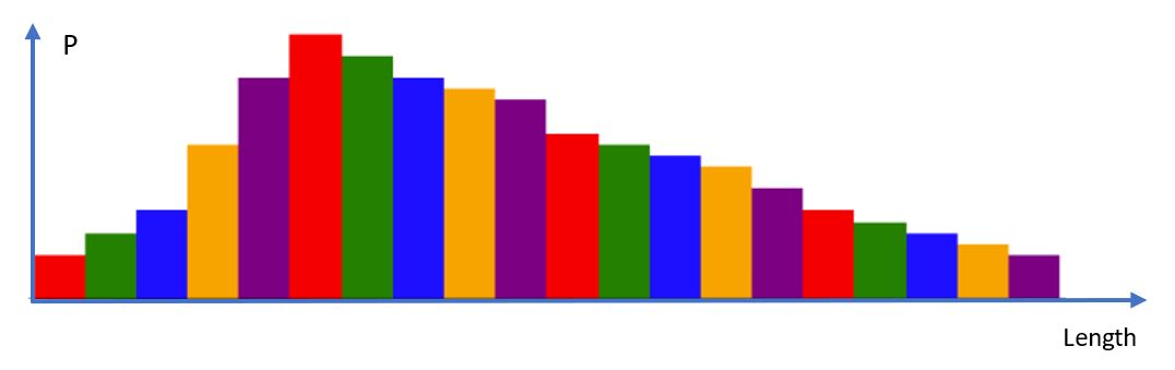
Figure 3
And if we want to make them still more granular, we can make the ranges even smaller, like 0.005 mm. And now we have all this information between 99.90 and 99.905 mm, between 99.905 and 99.91 mm, all the way to between 100.095 and 100.10 mm. And we can continue splitting these ranges and getting discrete distributions. And if we were to do this infinitely many times, then what we get is this: a continuous distribution. Imagine just a bunch of very, very skinny bars, infinitely many of them, that become just a curve.
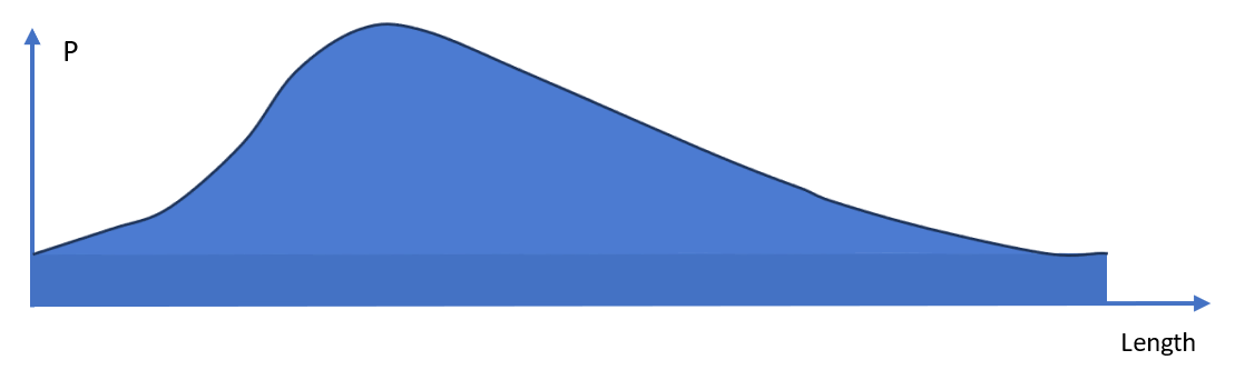
Figure 4
Now, in the discrete distribution, we had that the sum of heights has to be equal to 1. The sum of heights was the same as saying the blue area. So, in the continuous distribution, we have the same condition: the area under the curve is equal to 1. And that is a continuous probability distribution.
Probability Density Function
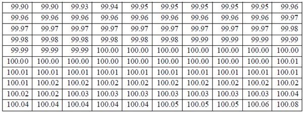
Let’s continue with same example of shaft length but with more concrete values and samples with length measurements. The nominal length of a shaft is 100 mm, with manufacturing tolerance is 0.1 mm, the actual length will be within the range of 100 ± 0.1 mm. The length measured vary from 99.90 mm to100.10 mm. 100 sample measurements of the length are given in Table. It ranges from 99.90 mm to100.10 mm, certain values occur more frequently than others. The values around the nominal length 100 mm occur with a higher chance than the values near both endpoints.
Table: Length of 100 Samples of shaft
If we divide the range [99.90, 100.10] into several equal segments and plot the number of values of the length that reside the segments, we will have a bar-like graph. This type of graph is called a histogram. It shows the frequency of the values that occur in different segments.
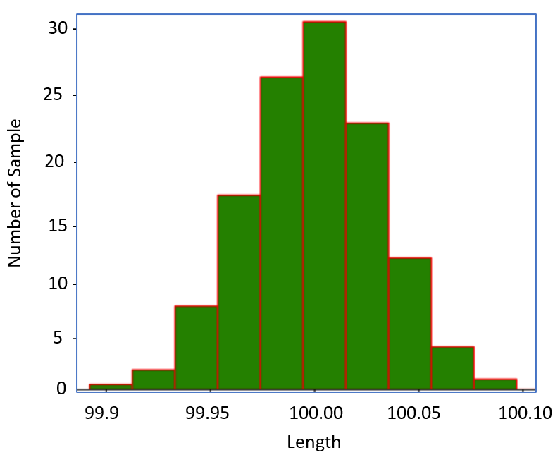
Figure 5
If we plot the number of samples (measurements) divided by the total number of measurements, we obtain a variant of the last histogram. As shown in Fig. below, the vertical axis represents the number of measurements within each segment divided by the total number of measurements (100).
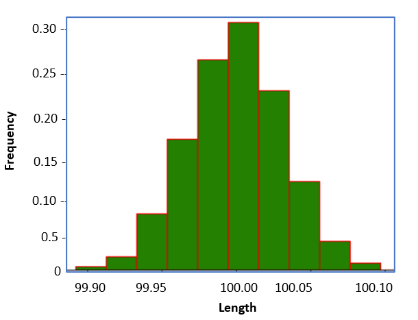
Figure 6
If we have more samples and use more intervals to divide the range of the length, the bars in the last Fig. will approach a smooth curve as shown in Fig. below. This curve is called a probability density function (pdf).
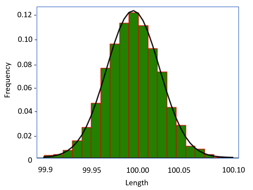
Figure 6
The pdf captures the chance property of a random variable as shown in Fig. below and fully describes a random variable.
- \(f(x)\) is used the denote a probability density function of random variable \(X\), where \(x\) is a realization (a specific value) of \(X\).
- The significance of the pdf is that \(f(x)dx\) is the probability that the random variable \(X\) is in the interval \([x, x + dx]\) (see Fig below), written as: \( P(x \leq X \leq x + dx) = f(x) \, dx \)
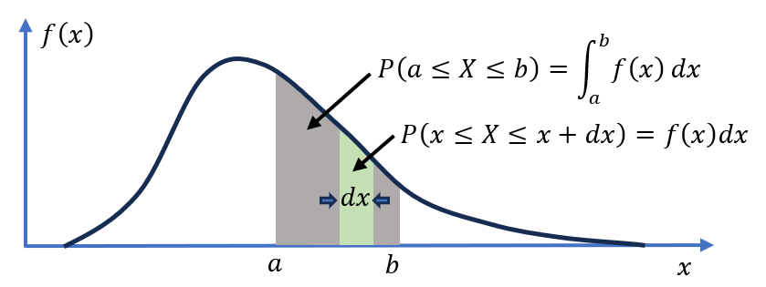
Figure 7
We can also determine the probability of \(X\) over a finite interval \([ a, b]\) as:
\( P(a \leq X \leq b) = \int_a^b f(x) \, dx \)
, also shown in figure above, which is the area underneath the curve of \(f(x)\) from \(x = a\) to \(x = b.\)
A pdf must be non-negative, i.e. \( f(x) \geq 0 \) and satisfies the following condition : \( \int_{-\infty}^{+\infty} f(x) \, dx = 1 \)
Example
Suppose the length of metal rods produced by a manufacturer follows a continuous distribution and probability density function (pdf)
is given by:
\(
f(x)=
\begin{cases}
\dfrac{1}{2}, & \text{for } 99 \le x \le 101 \\
0, & \text{otherwise}
\end{cases}
\)
Determine the probability that the rod's length is between 99.5 mm and 100.5 mm.
>Soln:
The probability is the area under the pdf curve between the specified limits as given.
\(P (99.5 ≤ X ≤ 100) = f(x) dx = f(x) × (100.5 − 99.5)\)
Since \(f(x) = 1/2\)
\(P (99.5 ≤ X ≤ 100.) = f(x) dx = f(x) × (100.5 − 99.5) = (1/2) ×1 =0.5\)
Conclusion: There is a 50% probability that a randomly selected rod will have a length between 99.5 mm and 100.5 mm.
One observation: In this example the density function remains constant for the specified ranges, for example PDF value is half for 99 ≤x ≤101. This is an example of uniform distribution, a type of continuous distribution.
Normal distribution, Exponential Distribution, and Uniform Distribution are examples of Continuous Probability Distributions. In the next article, we will focus on learning about the Normal distribution.