Let's continue with the case study of shaft length that we saw in the continuous distribution explanation. We were given lengths of 100 samples of shafts with a manufacturing tolerance of 0.1 mm, meaning the actual length will be within the range of 100 ± 0.1 mm. We divided the range [99.90, 100.10] into several equal segments and plotted the number of length values that reside in these segments. We had a bar-like graph called a histogram. It shows the frequency of the values that occur in different segments. We further modified it by dividing the frequency within each segment by the total sample count, which is 100. The final plot is shown below:
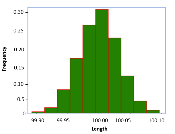
Figure 1
We can approximate this distribution with the bell-shaped curve shown below, and we will call this distribution as following Normal distribution.
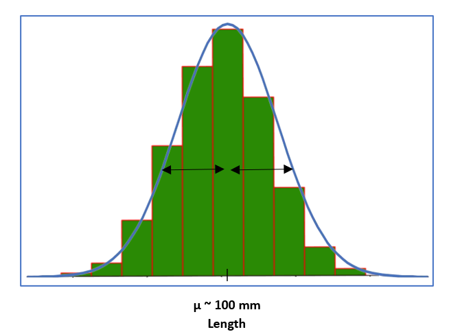
Figure 2
Now observe that most of the sample lengths are centered around a mean of approximately 100 mm and spread on both sides almost symmetrically. The ideal Normal distribution assumes a bell-shaped curve that is symmetrical around the mean value with a certain variance.
Normal random variables, also often called Gaussian random variables, are perhaps the most important ones in probability theory. They are prevalent in applications for two reasons: they have useful analytical properties, and they are the most common model for random noise. In general, they are a good model of noise or randomness whenever that noise is due to the addition of many small independent noise terms, and this is a very common situation in the real world.
We define normal random variables by specifying their PDFs as they are continuous distributions. We start with the simplest case, known as standard normal. The standard normal is denoted using the shorthand notation given below, and we will see shortly why this notation is used.
Standard Normal
\[ \mathcal{N}(0,1): \quad f_x(x) = \frac{1}{\sqrt{2\pi}} e^{-\frac{x^2}{2}} \]
This PDF is defined for all values of x, meaning x can be any real number i.e. this random variable can take values anywhere on the real line. Let us try to understand this formula.
It includes the exponential of \(-\frac{x^2}{2}\) (negative x squared over 2). If we are to plot the function \(\frac{x^2}{2}\) , it has a shape of the form shown below left, and it is centered at zero.
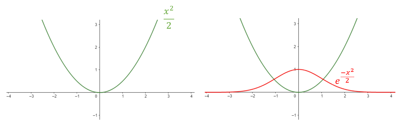
Figure 3
But then we take the negative exponential of this function. When you take the negative exponential, the value becomes small whenever \( \frac{x^2}{2} \)is large. Therefore, the negative exponential equals 1 when x is 0. As x increases and \(x^2\) also increases, the negative exponential decreases. Thus, we obtain a shape like the one shown on the top right in red colour, which is symmetrical on both sides.
finally, there is the constant --> \(\frac{1}{\sqrt{2\pi}}\): Where is this constant coming from? Well, there is a useful but somewhat complex calculus exercise that shows that the integral from minus infinity to plus infinity of \( e^{-\frac{x^2}{2}} \) is equal to \(\sqrt{2\pi}\) .
I.e. \( \int_{-\infty}^{+\infty} e^{-\frac{x^2}{2}} \, dx = \sqrt{2\pi} \)Now, we need a PDF that integrates to 1, meaning the area under the PDF curve should be 1. To achieve this, we include this constant in front of the expression so that the integral equals 1. This explains the presence of this particular constant.
What is the mean of this random variable?
Since x2 is symmetric around 0, and for this reason, the PDF itself is symmetric around 0. Therefore, by symmetry, the mean has to be equal to 0 or expectation: E[X]=0. This explains the entry zero in first position of standard normal notation: N (0,1).
How about the variance?
To calculate the variance, you need to solve a calculus problem involving integration by parts. After completing the calculation, you find that the variance is equal to 1or var(X)=1. This explains the entry one in the notation of standard normal: N (0,1).
General Normal (Gaussian) random variables
Let us now define general normal random variables. General normal random variables are specified their corresponding PDF as given below, which is more complex, and involves two parameters: \(\mu\), and \(\sigma^2\) , where sigma is a positive parameter, 𝞼>0.
Normal Random Variable
\[ \mathcal{N}(\mu, \sigma^2): \quad f_x(x) = \frac{1}{\sigma \sqrt{2\pi}} \, e^{-\frac{(x-\mu)^2}{2\sigma^2}} \]
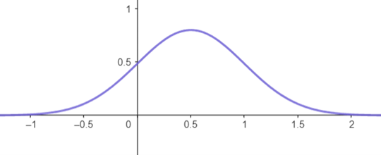
Figure 4
Once again, it will have a bell shape, but this bell is no longer symmetric around 0, and its width can be controlled.
To understand the form of this PDF, let's first focus on the exponent, just as we did with the standard normal case. The exponent is quadratic and is centered at x=μ. It vanishes when x=μ and becomes positive elsewhere. The curve is shown below in red. Taking the negative exponential of this quadratic results in a function that is highest at x=μ and decreases as we move further away from μ shown by purple colour.
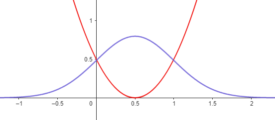
Figure 5
What is the mean of this random variable?
Since the exponent term is symmetric around μ, the PDF is also symmetric around μ, and therefore, the mean is also equal to μ, i.e. E[X]= μ.
What about the variance?
It turns out-- and this is a calculus exercise that we will omit-- that the variance of this PDF is equal to \(\sigma^2\), i.e. var(x) = \(\sigma^2\).
This explains the notation: \( \mathcal{N}(\mu, \sigma^2) \) , which indicates that we are dealing with a normal distribution with a mean of \(\mu\), and a variance of \(\sigma^2\)
Role of Sigma
We mentioned that in a general normal distribution, the width of the bell curve can be controlled, and this is the role of σ in the PDF. The figure below shows three normal curves with the same mean value of 0.5 but different σ values of 0.25, 0.5, and 0.75, respectively. We can clearly see that as σ increases, the width of the curve also increases.
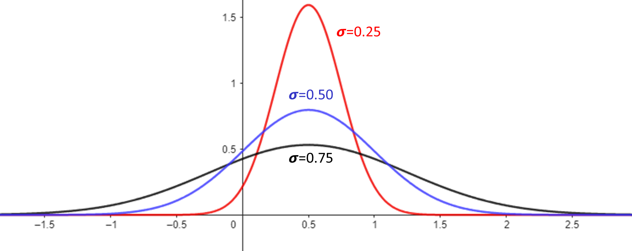
Figure 6
Examples of Normal Distribution
Many processes in nature result in events that follow a normal distribution. Height, weight, Test Scores, and even Measurement Errors are modeled by the normal distribution. In general, variables that can be modeled as a sum of many independent processes always follow normal distributions.
However, not all natural processes follow a normal distribution; some may follow other distributions depending on the underlying factors and their interactions viz. Earthquakes, Population Growth, Disease Outbreaks etc don’t follow normal distributions.
How does it fit into learning AIML?
Many machine learning algorithms have underlying assumptions of normal distributions. For example, Linear Regression and Logistic Regression assume normally distributed residuals and log-odds, respectively, for accurate inference. Gaussian Naive Bayes relies on the normal distribution for feature classification. The Central Limit Theorem supports using the normal distribution for sampling means. Techniques such as z-score normalization in feature scaling, and Gaussian Mixture Models for clustering often assume normality.
Additionally, neural networks use the normal distribution for weight initialization and batch normalization, while anomaly detection utilizes Gaussian models to identify deviations from normal behavior.
Thus, the normal distribution is pervasive in AI and ML, often operating behind the scenes.