Random Variables

We will see the formal definition of random variables later. First, let's start with a simple experiment of tossing a coin.

Tossing a coin results in either a head or a tail. Here, each possible outcome (getting a head or getting a tail) is an event. For a fair coin, the probability of getting a head or a tail is one-half.

\( P(H) = 0.5 \) and \(P(T) = 0.5 \)

Let's take a variable \(X\) and call it the number of heads. When we flip a coin, if we obtain heads, we get 1 head, and if we obtain tails, we get 0 heads.

X= Number of heads

Now writing the same probability of getting tail and head in this new framing of X as illustrated in Fig.1:

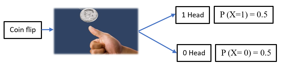
Figure 1

The probability of \(X = 1\) is the same as the probability of obtaining heads: \(P(X=1) = 0.5\)

The probability of \(X = 0\) is the same as the probability of obtaining tails: \(P(X=0) = 0.5\)

Here, X is a random variable as it can take either the value 1 or 0 randomly, with each value occurring roughly half of the time. Symbolically all possible outcomes/values that random variable can take are denoted by small \(x\), so \(x_1 = 1, x_2 = 0\). We can simply write \( X = \{x_1, x_2\} = \{1, 0\} \). There are only two values in sample space, \( Ω = \{1, 0\} \).

Note: \(P (X= x)\) is read as "the probability that the random variable \(X\) equals \(x​\)" and \(P (X = x) = 1/2 \) for either \(x = 0\) or \(1\).

In simpler terms, a random variable X assigns a real number to each outcome in the sample space \(Ω\).

Let’s see another example of rolling a fair six-sided die:

The sample space consists of all possible outcomes when rolling a six-sided die:\( Ω = \{1,2,3,4,5,6\}\).

Since the die is fair, each outcome is equally likely. Thus, the probability distribution of the random variable \(X\) is \(P (X = x) = 1/6 \) for \(x ∈ \{1,2,3,4,5,6\}.\)

Let’s see another example of 3 fair coin toss:

Define a random variable, X = Number of heads in 3-coin tosses.

Examine possible outcomes:

• All three coins land on the tail: \((ttt)\) Number of heads \((x) = 0\)
• At least one coin lands on the head and it can happen in 3 ways: \((tth, tht, htt)\) Number of heads \((x) = 1\)
• Two coins land on the head and it can happen in 3 ways:\((thh, hth, hht)\) Number of heads \((x) = 2\)
• All three coins land on the head: \((hhh)\) Number of heads \((x) = 3\)

Sample space, \(Ω = \{ttt, tth, tht, htt, thh, hth, hht, hhh \}; | Ω | = 8\)

Since all outcomes in the sample space are equiprobable(each with probability 1/8), the probability of a particular value of the random variable \( X \)depends on how many outcomes produce that value. Hence:

\( P(X = 0) = \frac{1}{8}, \, P(X = 1) = \frac{3}{8}, \, P(X = 2) = \frac{3}{8}, \, P(X = 3) = \frac{1}{8} \)

See the table below along with the histogram plot in Fig. 2 below:

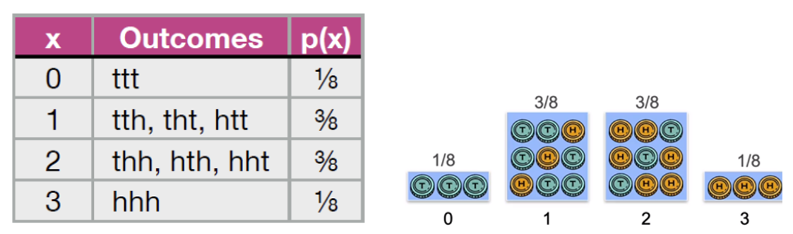
Figure 2

We have seen the three examples of random variables above, all of which are Discrete random variables. However, there are other types of random variables as well.

Examples of other type of random variables:

Amount of Rainfall in a Day:

The amount of rainfall in a day in a specific location is a continuous random variable. It can take any non-negative real value, from 0 mm on a dry day to several `mm` on a rainy day.

Speed of a Car on a Highway:

The speed of a car traveling on a highway is a continuous random variable. The speed can vary continuously over a range, such as between 0 km/h and the maximum speed limit, and can take any value within that range depending on traffic conditions and driver behaviour.

Blood Pressure Measurement:

The systolic blood pressure of a person is a continuous random variable. It can vary based on a person’s health, activity level, and other factors, and can take any value within a typical range, such as between 90 mmHg and 180 mmHg.

All of the above are examples of Continuous random variables.

Let’s compare both side by side.

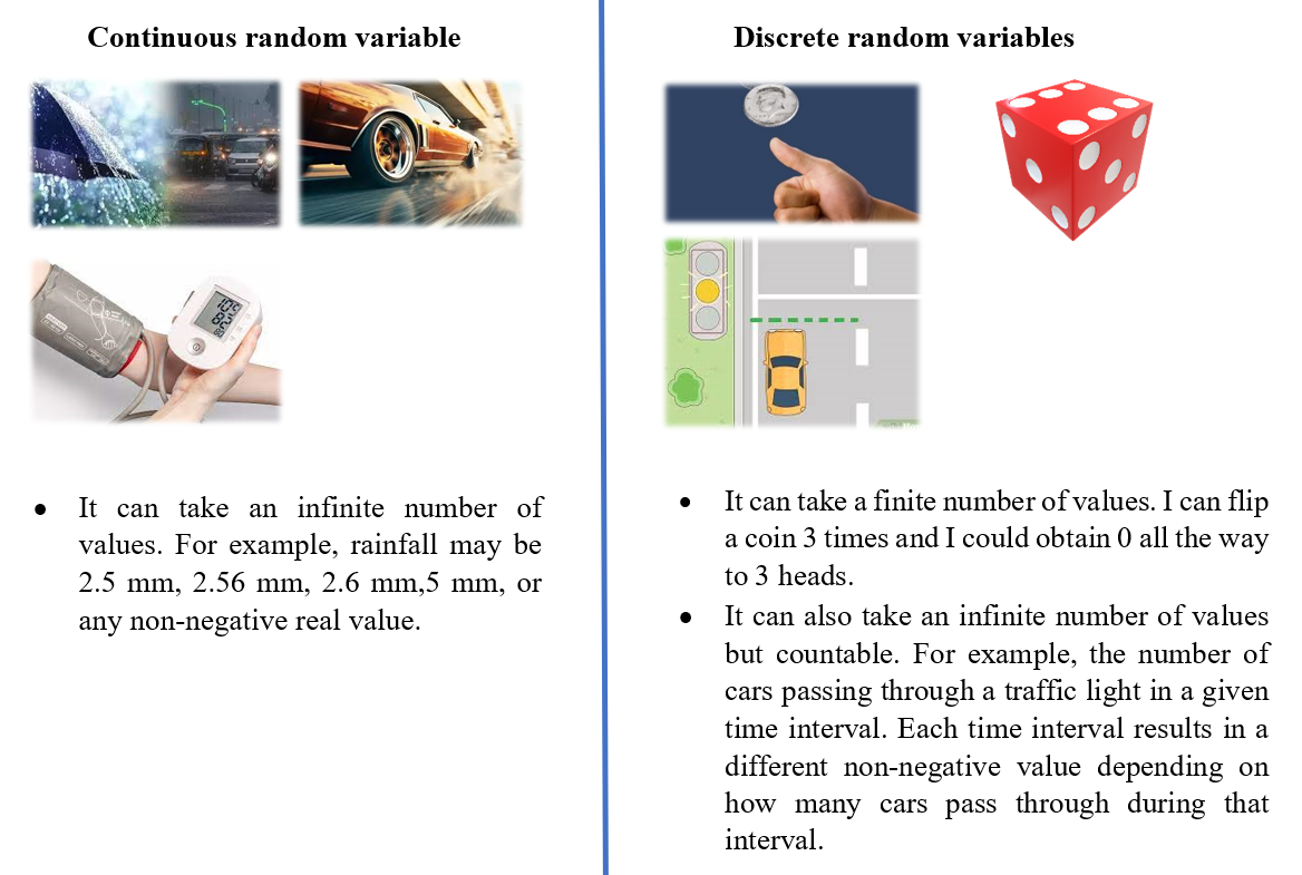
Figure 3

So, the values that a discrete random variable can take can be put in a list as 1, 2, 3, 4, 5, etc. Whereas the values that a continuous random variable takes cannot be put in a list because it's an entire interval.

What is the difference between these random variables and the ones seen in algebra and calculus?

The variables in algebra and calculus are deterministic, whereas the ones here are random. What is deterministic? For example, in algebra if \(x = 2\), or in the case of function \(f(x) = x^2\) the input always takes the same value. Once it's defined, it is fixed forever. However, a random variable is not like that. It can assume many values and is associated with an uncertain outcome. So deterministic variables are associated with a fixed outcome and random variables with an uncertain outcome, which is the primary distinction.

Terminologies

1. Probability Mass Function (PMF)

Definition: The probability mass function (PMF) applies to discrete random variables. It provides the probability that a discrete random variable is exactly equal to some value.

Mathematical Representation:\(P (X= x_i) = p(x_i)\), where \( p(x_i)\) is the probability that the random variable \(X\) takes the value \(x_i\)​.

Ex. For a fair six-sided die: \( P (X = x) = 1/6 \) for \(x ∈ \{1,2,3,4,5,6\}.\)

2. Probability Function

Definition: The term "probability function" is sometimes used interchangeably with "probability mass function" or "probability density function" (for continuous random variables), depending on the context. Generally, it refers to any function that gives the probability of occurrence of different possible outcomes of an experiment.

Types:

1. For Discrete Variables: The probability function is the PMF.
2. For Continuous Variables: The probability function is the Probability Density Function (PDF).

Details of probability density function will be covered in other part.